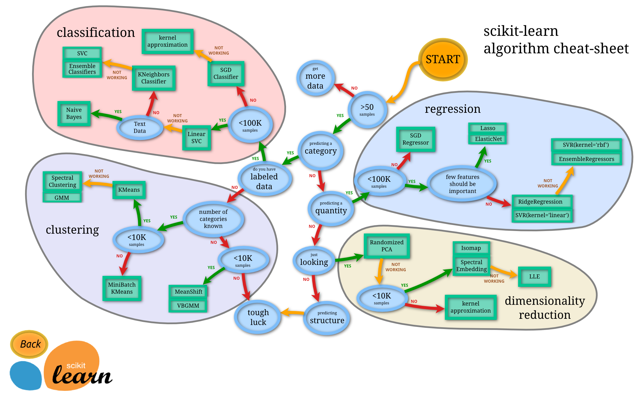
Scikit-Learn

Scikit-learn is an open source Python library that implements a range of machine learning, preprocessing, cross-validation and visualization algorithms using a unified interface.
Install and import Scikit-Learn
$ pip install scikit-learn
Scikit-learn Example
from sklearn import neighbors, datasets, preprocessing
from sklearn.model_selection import train_test_split
from sklearn.metrics import accuracy_score

# Load the Iris dataset
iris = datasets.load_iris()

# Split the dataset into features (X) and target (y)
X, y = iris.data[:, :2], iris.target

# Split the dataset into training and testing sets
X_train, X_test, y_train, y_test = train_test_split(X, y, random_state=33)

# Standardize the features using StandardScaler
scaler = preprocessing.StandardScaler().fit(X_train)
X_train = scaler.transform(X_train)
X_test = scaler.transform(X_test)

# Create a K-Nearest Neighbors classifier
knn = neighbors.KNeighborsClassifier(n_neighbors=5)

# Train the classifier on the training data
knn.fit(X_train, y_train)

# Predict the target values on the test data
y_pred = knn.predict(X_test)

# Calculate the accuracy of the classifier
accuracy = accuracy_score(y_test, y_pred)

# Print the accuracy
print("Accuracy:", accuracy)
Accuracy: 0.631578947368421
Loading The Data
from sklearn import datasets

# Load the Iris dataset
iris = datasets.load_iris()

# Split the dataset into features (X) and target (y)
X, y = iris.data, iris.target

# Print the lengths of X and y
print("Size of X:", X.shape) #  (150, 4)
print("Size of y:", y.shape) #  (150, )
Size of X: (150, 4)
Size of y: (150,)
Training And Test Data
# Import train_test_split from sklearn
from sklearn.model_selection import train_test_split

# Split the data into training and test sets with test_size=0.2 (20% for test set)
X, y = iris.data, iris.target
X_train, X_test, y_train, y_test = train_test_split(X, y, test_size=0.2, random_state=0)

# Print the sizes of the arrays
print("Size of X_train:", X_train.shape)
print("Size of X_test: ", X_test.shape)
print("Size of y_train:", y_train.shape)
print("Size of y_test: ", y_test.shape)
Size of X_train: (120, 4)
Size of X_test:  (30, 4)
Size of y_train: (120,)
Size of y_test:  (30,)
Create instances of the models
# Import necessary classes from sklearn libraries
from sklearn.linear_model import LogisticRegression
from sklearn.neighbors import KNeighborsClassifier
from sklearn.svm import SVC
from sklearn.cluster import KMeans
from sklearn.decomposition import PCA

# Create instances of supervised learning models
# Logistic Regression classifier (max_iter=1000)
lr = LogisticRegression(max_iter=1000)

# k-Nearest Neighbors classifier with 5 neighbors
knn = KNeighborsClassifier(n_neighbors=5)

# Support Vector Machine classifier
svc = SVC()

# Create instances of unsupervised learning models
# k-Means clustering with 3 clusters and 10 initialization attempts
k_means = KMeans(n_clusters=3, n_init=10)

# Principal Component Analysis with 2 components
pca = PCA(n_components=2)
Model Fitting
# Fit models to the data
lr.fit(X_train, y_train)
knn.fit(X_train, y_train)
svc.fit(X_train, y_train)
k_means.fit(X_train)
pca.fit_transform(X_train)

# Print the instances and models
print("lr:", lr)
print("knn:", knn)
print("svc:", svc)
print("k_means:", k_means)
print("pca:", pca)
lr: LogisticRegression(max_iter=1000)
knn: KNeighborsClassifier()
svc: SVC()
k_means: KMeans(n_clusters=3, n_init=10)
pca: PCA(n_components=2)
Prediction
# Predict using different supervised estimators
y_pred_svc = svc.predict(X_test)
y_pred_lr = lr.predict(X_test)
y_pred_knn_proba = knn.predict_proba(X_test)


# Predict labels using KMeans in clustering algorithms
y_pred_kmeans = k_means.predict(X_test)

# Print the results
print("Supervised Estimators:")
print("SVC predictions:", y_pred_svc)
print("Logistic Regression predictions:", y_pred_lr)
print("KNeighborsClassifier probabilities:\n", y_pred_knn_proba[:5],"\n     ...")

print("\nUnsupervised Estimators:")
print("KMeans predictions:", y_pred_kmeans)
Supervised Estimators:
SVC predictions: [2 1 0 2 0 2 0 1 1 1 2 1 1 1 1 0 1 1 0 0 2 1 0 0 2 0 0 1 1 0]
Logistic Regression predictions: [2 1 0 2 0 2 0 1 1 1 2 1 1 1 1 0 1 1 0 0 2 1 0 0 2 0 0 1 1 0]
KNeighborsClassifier probabilities:
 [[0. 0. 1.]
 [0. 1. 0.]
 [1. 0. 0.]
 [0. 0. 1.]
 [1. 0. 0.]]
     ...

Unsupervised Estimators:
KMeans predictions: [2 2 0 1 0 1 0 2 2 2 1 2 2 2 2 0 2 2 0 0 2 2 0 0 2 0 0 2 2 0]
Preprocessing The Data
Standardization
from sklearn.preprocessing import StandardScaler

# Create an instance of the StandardScaler and fit it to training data
scaler = StandardScaler().fit(X_train)

# Transform the training and test data using the scaler
standardized_X = scaler.transform(X_train)
standardized_X_test = scaler.transform(X_test)

# Print the variables
print("\nStandardized X_train:\n", standardized_X[:5],"\n     ...")
print("\nStandardized X_test:\n", standardized_X_test[:5],"\n     ...")
Standardized X_train:
 [[ 0.61303014  0.10850105  0.94751783  0.736072  ]
 [-0.56776627 -0.12400121  0.38491447  0.34752959]
 [-0.80392556  1.03851009 -1.30289562 -1.33615415]
 [ 0.25879121 -0.12400121  0.60995581  0.736072  ]
 [ 0.61303014 -0.58900572  1.00377816  1.25412853]]
     ...

Standardized X_test:
 [[-0.09544771 -0.58900572  0.72247648  1.5131568 ]
 [ 0.14071157 -1.98401928  0.10361279 -0.30004108]
 [-0.44968663  2.66602591 -1.35915595 -1.33615415]
 [ 1.6757469  -0.35650346  1.39760052  0.736072  ]
 [-1.04008484  0.80600783 -1.30289562 -1.33615415]]
     ...
Normalization
from sklearn.preprocessing import Normalizer
scaler = Normalizer().fit(X_train)
normalized_X = scaler.transform(X_train)
normalized_X_test = scaler.transform(X_test)

# Print the variables
print("\nNormalized X_train:\n", normalized_X[:5],"\n     ...")
print("\nNormalized X_test:\n", normalized_X_test[:5],"\n     ...")
Normalized X_train:
 [[0.69804799 0.338117   0.59988499 0.196326  ]
 [0.69333409 0.38518561 0.57777841 0.1925928 ]
 [0.80641965 0.54278246 0.23262105 0.03101614]
 [0.71171214 0.35002236 0.57170319 0.21001342]
 [0.69417747 0.30370264 0.60740528 0.2386235 ]]
     ...

Normalized X_test:
 [[0.67767924 0.32715549 0.59589036 0.28041899]
 [0.78892752 0.28927343 0.52595168 0.13148792]
 [0.77867447 0.59462414 0.19820805 0.02831544]
 [0.71366557 0.28351098 0.61590317 0.17597233]
 [0.80218492 0.54548574 0.24065548 0.0320874 ]]
     ...
Binarization
import numpy as np
from sklearn.preprocessing import Binarizer

# Create a sample data array
data = np.array([[1.5, 2.7, 0.8],
                 [0.2, 3.9, 1.2],
                 [4.1, 1.0, 2.5]])

# Create a Binarizer instance with a threshold of 2.0
binarizer = Binarizer(threshold=2.0)

# Apply binarization to the data
binarized_data = binarizer.transform(data)

print("Original data:")
print(data)
print("\nBinarized data:")
print(binarized_data)
Original data:
[[1.5 2.7 0.8]
 [0.2 3.9 1.2]
 [4.1 1.  2.5]]

Binarized data:
[[0. 1. 0.]
 [0. 1. 0.]
 [1. 0. 1.]]
Encoding Categorical Features
from sklearn.preprocessing import LabelEncoder

# Sample data: categorical labels
labels = ['cat', 'dog', 'dog', 'fish', 'cat', 'dog', 'fish']

# Create a LabelEncoder instance
label_encoder = LabelEncoder()

# Fit and transform the labels
encoded_labels = label_encoder.fit_transform(labels)

# Print the original labels and their encoded versions
print("Original labels:", labels)
print("Encoded labels:", encoded_labels)

# Decode the encoded labels back to the original labels
decoded_labels = label_encoder.inverse_transform(encoded_labels)
print("Decoded labels:", decoded_labels)
Original labels: ['cat', 'dog', 'dog', 'fish', 'cat', 'dog', 'fish']
Encoded labels: [0 1 1 2 0 1 2]
Decoded labels: ['cat' 'dog' 'dog' 'fish' 'cat' 'dog' 'fish']
Imputing Missing Values
import numpy as np
from sklearn.impute import SimpleImputer

# Sample data with missing values
data = np.array([[1.0, 2.0, np.nan],
                 [4.0, np.nan, 6.0],
                 [7.0, 8.0, 9.0]])

# Create a SimpleImputer instance with strategy='mean'
imputer = SimpleImputer(strategy='mean')

# Fit and transform the imputer on the data
imputed_data = imputer.fit_transform(data)

print("Original data:")
print(data)
print("\nImputed data:")
print(imputed_data)
Original data:
[[ 1.  2. nan]
 [ 4. nan  6.]
 [ 7.  8.  9.]]

Imputed data:
[[1.  2.  7.5]
 [4.  5.  6. ]
 [7.  8.  9. ]]
Generating Polynomial Features
import numpy as np
from sklearn.preprocessing import PolynomialFeatures

# Sample data
data = np.array([[1, 2],
                 [3, 4],
                 [5, 6]])

# Create a PolynomialFeatures instance of degree 2
poly = PolynomialFeatures(degree=2)

# Transform the data to include polynomial features
poly_data = poly.fit_transform(data)

print("Original data:")
print(data)
print("\nPolynomial features:")
print(poly_data)
Original data:
[[1 2]
 [3 4]
 [5 6]]

Polynomial features:
[[ 1.  1.  2.  1.  2.  4.]
 [ 1.  3.  4.  9. 12. 16.]
 [ 1.  5.  6. 25. 30. 36.]]
Classification Metrics
from sklearn.metrics import accuracy_score, classification_report, confusion_matrix

# Accuracy Score
accuracy_knn = knn.score(X_test, y_test)
print("Accuracy Score (knn):", knn.score(X_test, y_test))

accuracy_y_pred = accuracy_score(y_test, y_pred_lr)
print("Accuracy Score (y_pred):", accuracy_y_pred)

# Classification Report
classification_rep_y_pred = classification_report(y_test, y_pred_lr)
print("Classification Report (y_pred):\n", classification_rep_y_pred)

classification_rep_y_pred_lr = classification_report(y_test, y_pred_lr)
print("Classification Report (y_pred_lr):\n", classification_rep_y_pred_lr)

# Confusion Matrix
conf_matrix_y_pred_lr = confusion_matrix(y_test, y_pred_lr)
print("Confusion Matrix (y_pred_lr):\n", conf_matrix_y_pred_lr)
Accuracy Score (knn): 0.9666666666666667
Accuracy Score (y_pred): 1.0
Classification Report (y_pred):
               precision    recall  f1-score   support

           0       1.00      1.00      1.00        11
           1       1.00      1.00      1.00        13
           2       1.00      1.00      1.00         6

    accuracy                           1.00        30
   macro avg       1.00      1.00      1.00        30
weighted avg       1.00      1.00      1.00        30

Classification Report (y_pred_lr):
               precision    recall  f1-score   support

           0       1.00      1.00      1.00        11
           1       1.00      1.00      1.00        13
           2       1.00      1.00      1.00         6

    accuracy                           1.00        30
   macro avg       1.00      1.00      1.00        30
weighted avg       1.00      1.00      1.00        30

Confusion Matrix (y_pred_lr):
 [[11  0  0]
 [ 0 13  0]
 [ 0  0  6]]
Regression Metrics
from sklearn.metrics import mean_absolute_error, mean_squared_error, r2_score

# True values (ground truth)
y_true = [3, -0.5, 2]

# Predicted values
y_pred = [2.8, -0.3, 1.8]

# Calculate Mean Absolute Error
mae = mean_absolute_error(y_true, y_pred)
print("Mean Absolute Error:", mae)

# Calculate Mean Squared Error
mse = mean_squared_error(y_true, y_pred)
print("Mean Squared Error:", mse)

# Calculate R² Score
r2 = r2_score(y_true, y_pred)
print("R² Score:", r2)
Mean Absolute Error: 0.20000000000000004
Mean Squared Error: 0.040000000000000015
R² Score: 0.9815384615384616
Clustering Metrics
from sklearn.metrics import adjusted_rand_score, homogeneity_score, v_measure_score

# Adjusted Rand Index
adjusted_rand_index = adjusted_rand_score(y_test, y_pred_kmeans)
print("Adjusted Rand Index:", adjusted_rand_index)

# Homogeneity Score
homogeneity = homogeneity_score(y_test, y_pred_kmeans)
print("Homogeneity Score:", homogeneity)

# V-Measure Score
v_measure = v_measure_score(y_test, y_pred_kmeans)
print("V-Measure Score:", v_measure)
Adjusted Rand Index: 0.7657144139494176
Homogeneity Score: 0.7553796021571243
V-Measure Score: 0.8005552543570766
Cross-Validation
# Import necessary library
from sklearn.model_selection import cross_val_score

# Cross-validation with KNN estimator
knn_scores = cross_val_score(knn, X_train, y_train, cv=4)
print(knn_scores)

# Cross-validation with Linear Regression estimator
lr_scores = cross_val_score(lr, X, y, cv=2)
print(lr_scores)
[0.96666667 0.93333333 1.         0.93333333]
[0.96 0.96]
Grid Search
# Import necessary library
from sklearn.model_selection import GridSearchCV

# Define parameter grid
params = {
    'n_neighbors': np.arange(1, 3),
    'weights': ['uniform', 'distance']
}

# Create GridSearchCV object
grid = GridSearchCV(estimator=knn, param_grid=params)

# Fit the grid to the data
grid.fit(X_train, y_train)

# Print the best parameters found
print("Best parameters:", grid.best_params_)

# Print the best cross-validation score
print("Best cross-validation score:", grid.best_score_)

# Print the accuracy on the test set using the best parameters
best_knn = grid.best_estimator_
test_accuracy = best_knn.score(X_test, y_test)
print("Test set accuracy:", test_accuracy)
Best parameters: {'n_neighbors': 1, 'weights': 'uniform'}
Best cross-validation score: 0.9416666666666667
Test set accuracy: 1.0